1. Introduction
Live migration is an important technique enabling elastic management of virtualized resources. Virtual machines (VMs) can be migrated transparently to a physically distinct host with live migration. However, live migration often involves an iterative transfer of the VM’s memory and consumes a significant amount of network I/O resources and could disrupt services running in the VM. The performance of a live migration is highly dependent on the workload running in the migrated VM, the available resources on the source and destination server, and co-located services running on the same hosts. Due to the large parameter space related to live migration performance, an accurate prediction of live migration is a challenging problem. Previous efforts to predict live migration metrics are mainly based on analytic approaches, but are limited in applicability or sacrifice accuracy due to the complexity of the various live migration algorithms and the vast parameter space of live migration.
Machine learning (ML) is a good candidate to tackle this problem. The main challenge when designing an ML model is preparing a high-quality data set. A good data set must cover the entire parameter space and include a sufficient number of samples. The parameters (or input features) are selected by a domain expert.
In this document, we describe our VM live migration data set containing over 40,000 live migration samples that have been gathered over a period of several months in our internal cluster. We briefly discuss how we have designed an accurate ML model using the dataset and provide the code used for training and prediction.
Getting access to the dataset / ML model source code
The dataset is provided to interested researchers to perform their own analyses. To get access to the dataset, contact changyeon@csap.snu.ac.kr.
If you make use of the dataset, we ask you to reference our paper "A Machine Learning Approach to Live Migration Modeling" presented at the 2017 ACM Symposium of Cloud Computing. Here's the relevant bibtex entry.
For the further detail about the dataset, please read through this document.
2. The cluster

The cluster which used for the dataset generation consists of four identical machines which feature 4-core Skylake i5-6600 processor, 16GB memory, 1 gigabit dedicated NIC for the migration traffic, and a shared storage equipped with SSDs connected through NFS protocol. The storage traffic is also severed by a dedicated NIC in each server.
P.S. We are building a new dataset on a more large scale and the heterogeneous cluster which consists of various generations of Intel and AMD processors. Also, we adjusted the processor frequencies to simulate a more heterogeneous hardware environments.
3. The Dataset
The live migration data set contains 40,000+ migration samples have gathered for several months in CSAP lab cluster. The dataset is targeted to train a general model for VM live migration, so the workloads running in our cluster were prepared to cover wide parameter space of cloud workloads. In summary, we have run 37 unique applications and benchmark workloads.
2.1 The synthetic workload generator
To cover large parameter space, we have designed a synthetic workload generator. The workload generator is designed especially to explore performance characteristics of various live migration algorithms.
2.2 The workloads from applications and benchmark suites
| Workload | Description |
|---|---|
| Memcached | Memcached is a NoSQL database which has been deployed in a large number of the production environment to accelerate latency critical services. We run memcached in VMs and configure it with a range of random parameters to cover a various VM workload parameter space. To stress the memcached server, we run clients in a dedicated physical machine in the same cluster. The memcached request traffic is served by a dedicated NIC on the physical server which the memcached VM is deployed. Yahoo Cloud Serving Benchmark is used for the client software. |
| OLTPbenchmark | OLTPbenchmark is a sum of various workloads that simulate online transaction processing scenarios. We employed MySQL database in each VM to serve data and run the clients in a dedicated physical machine in the cluster. TPC-C, Wikipedia, and Facebook (TODO: verify the selected benchmark) workloads are selected for the workloads in the dataset. You can find more detail in the benchmark suite in the link. |
| SPECWeb2009 | SPECWeb is a benchmark which designed to measure web server performance. We deployed LAMP (Linux, Apache, MySQL, and PHP) in the VM for the test and built the environment using SPECWeb2009 script. SPECWeb20009 clients run on a dedicated physical server in the cluster, and the request traffic is served by a dedicated 1 gigabit NIC on each server. You can find more detail in the benchmark suite in the link. |
| Parsec | Parsec, a benchmark suite is designed to test system performance for emerging multicore applications. We selected blackscholse, bodytrack, dedup, and fluidanimate for the VM workloads. To generate diverse characteristic workloads, we dynamically configured thread numbers for an execution and each run. You can find more detail in the benchmark suite in the link. |
| Dacapo | Dacapo is a benchmark suite including the set of Java applications that have non-trivial memory loads. We selected avrora, eclipse, fop, h2, and pmd workloads in the suite for the VM workloads. Dacapo benchmark support parameters that input size and the number of thread for execution. We also dynamically changed the parameters for each run to get diverse workloads. You can find more detail in the benchmark suite in the link. |
| Gzip | Bzip workloads is a system administration workloads which compress large log data of a system. We run Gzip workloads which compress 10GB of ukwikipedia dump data in a VM. To get diverse workloads we changed compressibility parameter for each which makes a user can tradeoff between compression quality and size. |
| Mplayer | Mplayer workload is deployed to simulate online video streaming service which widely used lately in production. We prepared open source movies and downloaded YouTube video for the workloads. The movie files are placed in the VM and dynamically changed the video for play in each different run. |
| Idle | In addition to the realistic workloads, the dataset also contains idle workloads which only occupy some size of memory but do not execute any application inside of the VM. To make diverse idle VMs that each VM occupies different size of memory, we allocate memory inside of a VM and tough the every memory location once. With the simple steps, the VM process reservation size (size of physically mapped memory of a process) is increased as the had allocated memory in the VM. |
4. Structure of the Dataset
The dataset is a CSV file including 40,753 (TODO) lines. The first line is the metadata of each column of the row and the following rows are mapped to a unique data points which composed as one dimension feature vector.
Here is a sample of the metadata and a data point.
|
capability,workload_type,VM_size,VM_pdr,VM_wss,VM_wse,VM_nwse,VM_mwpp,VM_pmu_instr,VM_ptr,VM_cpu_util,VM_net_util,src_cpu_avail,dst_cpu_avail,src_mem_avail,dst_mem_avail,qemu_tt,qemu_dt,qemu_td,performance,used_cpu_src,used_mem_src |
In the following subsection, we are going to explain full details of each feature of the dataset.
4.1 The features
All live migration algorithms involve memory transfer from the source machine to the destination machine, and memory use pattern of a VM is highly affect the performance of live migration. Thus, we designed the feature space to cover various memory use pattern characteristics of a VM. We have analyzed more than ten different live migration techniques and carefully designed the feature set can cover as many as algorithms. We have validated the model to five live migration algorithms which are available in QEMU but we sure that the features still applicable to other algorithms at least the migration technique exploit memory use pattern of a VM.
| Feature | Description | Source |
|---|---|---|
| Migration algorithm (capability) | The migration technique which used to migrate the workload of the data point. Available values are integer values from 0.0 to 4.0. For each value is mapped to a migration technique. Here is the full detail of the mapping. 0: original precopy, 1: CPU throttling, 2: Delta-compression, 3: Data-compression, 4: post-copy. | VMM |
| Workload type (workload_type) | The name of the workload used to generate the data point. The available range of value is an integer from 0 to 9. Each integer value is mapped to a unique application. Here is the full detail of the mapping. 0: synthetic workload, 1: idle workload … (TODO: complete the mapping information) | |
| VM size (VM_size) | The total amount of VM memory that mapped to physical memory. Note that, the zero pages are not included in the VM_size. QEMU can efficiently identify zero pages of a VM, and it avoids to send the zero pages when migrating a VM, thus excluding zero pages in VM size will make the feature more relevant in the modeling. | |
| Page dirty rate (VM_pdr) | The average number of pages modified for a given period. The number of modified pages in the dataset is collected at every second for 20 seconds, and the page dirty rate is the average of the twenty samples. | |
| Working set size (VM_wss) | The size of modified pages for the period (20 seconds in the dataset). | |
| Working set entropy (VM_wse) | The entropy of the working set memory. Entropy is a value which ranges from 0 to 1. A higher value of entropy denotes that the compressibility of data is low. The entropy is computed for each page in a working set, and we took average to get the final value. Byte-level histogram of a page is required to compute entropy, and it is a relatively costly feature to get. The entropy is highly related to the performance of data compression based live migration algorithms. | |
| Modified words per page (VM_mwpp) | The number of modified words per page. We gathered twenty samples which collected at every second. The page size is 4096 bytes, and the word size is 1 byte in our environment. Thus the maximum number of VM_mwpp is 4096. This metric is important for some compression based techniques which exploit previous data that the destination already has. For example, if we know the destination already has the page of the previous version, the sender only needs to modified part of the data. XBZRLE (Xor Based Zero Run Length Encoding) technique in QEMU apply XOR with old and new data, then compress it using run length encoding. We can expect higher compression rate when the VM_mwpp is high. | |
| Instructions per second (IPS, VM_pmu_instr) | The IPS is the number of retired instructions executed by the VM. If we assume that a VM workload is stable, we can use the IPS as a performance metric of the VM. The IPS can easily be measured outside of the VM. Most of modern Intel and AMD processors provide hardware performance event counter and Linux perf utility provide an easy interface to count per process performance counter event. We attach perf to VM process and count the IPS. | |
| Page transfer rate (VM_ptr) | The page transfer rate is the network bandwidth reserved for a migration traffic. QEMU provides an interface to limit the bandwidth will be used for live migration. All migrations in the dataset guaranteed the requested bandwidth during a live migration. Each machine in our test environment has dedicated NIC for migration traffic; thus the applications and storage traffic do not compete for the bandwidth. | |
| CPU utilization of VM (VM_cpu_util) | The CPU utilization of VM is the average CPU utilization of a VM for a given period in percent. We measured the average CPU utilization for twenty seconds before we trigger a migration. We use Linux utility top to monitor process CPU utilization. | |
| Network utilization of VM (VM_net_util) | The network utilization of VM is the average network utilization of the network interface which attached to the VM in percent. We also measured the value for twenty seconds before we trigger a migration. | |
| CPU utilization on host (SRC|DST.CPU) | The CPU utilization of source and destination hosts are the average amounts of CPU resource at the time of migration. We use top command to measure the value and measure the CPU utilization at one-second interval twenty seconds before we trigger a migration. | |
| Memory utilization on host (SRC|DST.MEM) | The memory utilization of source and destination hosts are the used memory at the time of migration in MB. We took the peak memory utilization during twenty seconds before we trigger a migration. The total memory size of a host is 16GB. | |
| Weighted relative page transfer rate (R.PTR) | Weighted relative page transfer rate is a composed feature which important to predict time-related prediction metrics such total migration time and downtime. This feature is important because the page transfer rate should be interpreted regarding the migrating workloads. Especially the impact of the PTR is large at the boundary of PDR that is the reason why we apply square to (PDR/PTR) in the formula for R.PTR. | |
| Non-working set size (NWSS) | The non-working size is the “cold” region of a VM’s memory. The size of hot and cold regions affect to migration performance significantly because hot pages are likely to transfer to the destination many times and cold pages do not. Computing this feature is trivial, the value is computed by subtracting the working set size from the VM size. | |
| Benefit of delta compression (DLTC.BF) | The Benefit of delta compression is a composed feature which designed to easy to fit on the model for the delta compression technique. This feature can be treated as the weighted working set size that uses MWPP as the coefficient. | |
| Benefit of CPU throttling (THR.BF) | The benefit of CPU throttling is a key feature which important to the effectiveness of CPU throttling technique. The major finding of CPU throttling throughout our experiences was that it does not guarantee the finish of migration. Migration is infinitely continued when the amount of memory in iterative pre-copy is above than a threshold. CPU throttling force to decrease the speed of a VCPU to make the amount of transferred memory in iteration below the threshold. However, it does not always work when a CPU is very effectively dirtying pages of a VM. One clear example is just modifying a byte of every page with very little CPU time. This feature can be used as an indicator that the CPU throttling can make the workload converge of not. | |
| Compressed size of WSS (E.WSS) | The compressed size of WSS is expected the size of the working set when we compress the page with data compression algorithm used in QEMU. It is important to compression based algorithms because E.WSS is a number of bytes actually transferred to the destination. | |
| Compressed size of NWSS( E.NWSS) | The compressed size of NWSS is expected the size of the non working set when we compress the page with data compression algorithm used in QEMU. It is important to compression based algorithms because E.NWSS is a number of bytes actually transferred to the destination. |
4.2 Prediction targets
The current model predicts total six performance metrics which are useful to manage SLAs of services in a data center. The model can be extended with little effort. For example, if you want to make the model predict additional power consumption of migration, you can just reuse the current feature set. However, it requires new data points which containing power consumption information.
| Metric | Description | Source |
|---|---|---|
| Total migration time (qemu_tt) | The total migration time of VM measured in QEMU. We took the value from the “info migrate” result in QEMU hmp monitor. After a successful migration, you can get the value through the command. | |
| Downtime (qemu_dt) | The downtime of the VM in milliseconds. We took the value from the “info migrate” result in QEMU hmp monitor. After a successful migration, you can get the value through the command. | |
| Total transferred data (qemu_td) | The total transferred data in bytes of the VM. We took the value from the “info migrate” result in QEMU hmp monitor. After a successful migration, you can get the value through the command. | |
| Performance degradation of VM (performance) | We measure the VM performance using a black box metric that “number of retired instructions per a second” (IPS). | |
| Additional CPU consumption during the migration | The additional CPU consumption during the migration is computed by subtracting the host CPU utilization during the profiling phase from the host CPU utilization during the migration. It does not accurately measure the additional CPU utilization of live migration algorithm, but it is known that data center workloads are quite stable. Thus we can treat the increased CPU utilization of a host for this metric. | |
| Additional memory consumption during the migration | The additional memory consumption during the migration is computed by subtracting the host memory utilization during the profiling phase from the host memory utilization during the migration. It does not accurately measure the additional memory utilization of live migration algorithm, but it is known that data center workloads are quite stable. Thus we can treat the increased memory utilization of a host for this metric. |
5. Statistics of the dataset
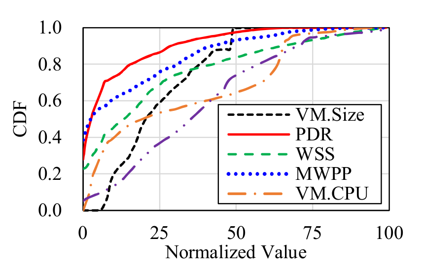
The dataset cover wide space of application workloads to train the migration model to general cases as much as possible. The above figure shows CDF of the key input features such as VM size, page dirty rate, working set size, modified words per page, and CPU utilization of a VM. As shown in the figure, the input feature in the dataset is widely spread throughout the feature spaces.
6. 512 Migration Dataset
In addition to the 40,000 migration dataset, we provide another dataset that contains migration result of 512 workloads for each migration algorithm. We configure the experiment script to reproduce the cluster status for a given seed number; then we migrate the same VM with the five different migration algorithms. Thus we can fairly compare the live migration algorithms for various workloads. In the SoCC’17 paper, we used the 512 migration dataset to show that the benefit of each live migration algorithm is highly dependent on a given workload, and there is no always winning one algorithm. Also used the dataset to show a machine-learned model can be used to as a guide to select proper migration algorithm for a given workload. You can find the detail in Section 8 Model-guided VM migration in the SoCC’17 paper.
6.1 Structure of the dataset
Only two additional column is added to 512 migration dataset that seed_number and sequence_number for each row, you can treat the tuple of two values as a unique identifier of the workload.
7. Analyzing the Dataset
Pre-requisite: python3 and scikit-learn 0.18
We provide a sample source code which performs training and prediction on the dataset. The script is written in python3 and uses scikit-learn for training and validation.
7.1 Fit the data on SVR model with bagging.
The following source code fits the dataset on SVR model with bagging. The source code reproduces the result of Table 2. in the SoCC’17 paper.
|
#!/usr/bin/env python3
# """ schema """
def build_features(features):
VM_size = features[0]
if VM_wss * ((VM_pdr / VM_ptr)**2) < VM_wss:
VM_nwss = VM_size - VM_wss return features
def load_dataset(dataset_path):
with open(dataset_path, 'r') as fp:
rows = rows[1:]
size = 0 return schema, capabilities, workload_types, X, y, size
def evaluate(metric, pv, tv):
abs_err = []
MAE = mean(abs_err)
min_abs_err = max(abs_err)
non_zero_abs_err = []
for i in range(len(rel_err)):
gMAE = gmean(non_zero_abs_err) return gMAE, gMRE
def modeling(schema, capabilities, workload_types, X, y, size, model='Bagging'):
if model == 'Linear':
predicted = cross_val_predict(clf, X_standard, y_standard.ravel(), cv=10, n_jobs=10)
if __name__ == "__main__": |